
Introduction: the memory bottleneck
as models get larger and larger a single device won’t get us through training although the largest portion of memory is often not occupied by the model parameters themselves but by stored intermediate values required for training
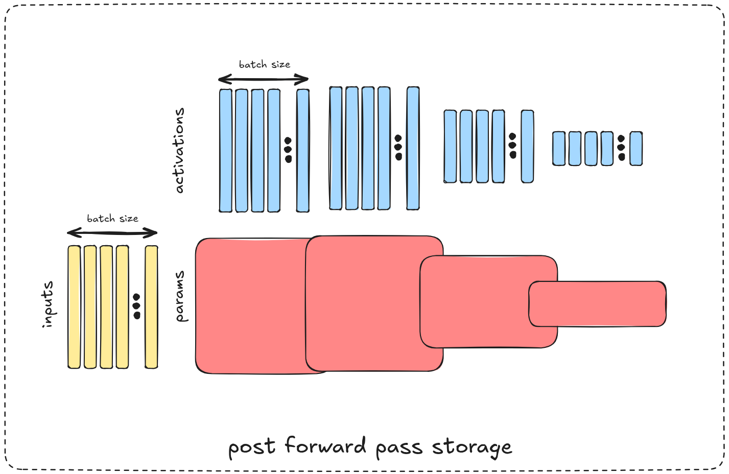
to better understand the problem, let’s consider a simple layers MLP each with 128 perceptrons and 128 as the input dimension, assuming all used values in float32 and ignoring biases for simplicity
(we’ll also ignore the optimizer state for simplicity)
the model parameters occupy:
on the other hand the intermediate activation values to store during training needed to compute the gradients during backpropagation for each sample in the batch occupy:
in this case whether the memory space occupied by activations (saved intermediate values) will over-weight the model’s params or not depends on whether the batch size exceeds the model width 128
in models where the same params / tensors are used for multiple operations (e.g residual connections, per token operations) the parameters themselves won’t grow in size with the sequence length (:number of tokens) but the activations will sure do, as a result the activations memory space will easily over weight the parameters memory space (by orders of magnitude in some applications)

Data Parallel
one of the simplest solutions for such encounter, on a single device, would be gradient accumulation which is computing the gradient of the entire batch on multiple steps (splitting the batch over n micro-batches and accumulating the gradients on each backward pass) which will require n times less memory space for activations by transforming the computing the gradients of the entire batch into a sequential process (computing the gradients for the first [batch / n] samples, the second [batch / n] samples, …)
Using multiple devices we can simply optimize that through parallelization, still computing the gradient of a single micro-batch (:[batch / n] samples) per run but instead of computing them in a sequence on the same device we would clone the entire model on n different devices and run a micro-batch on each, as a result, after a single time step we have the gradients for all samples, computed independently and sharded across devices. These gradients are then synchronized via a collective
All-Reduce
operation, which reduces (sums) the per-device gradients and distributes the averaged result back to every model replica, after which each device applies the optimizer update using this shared gradient.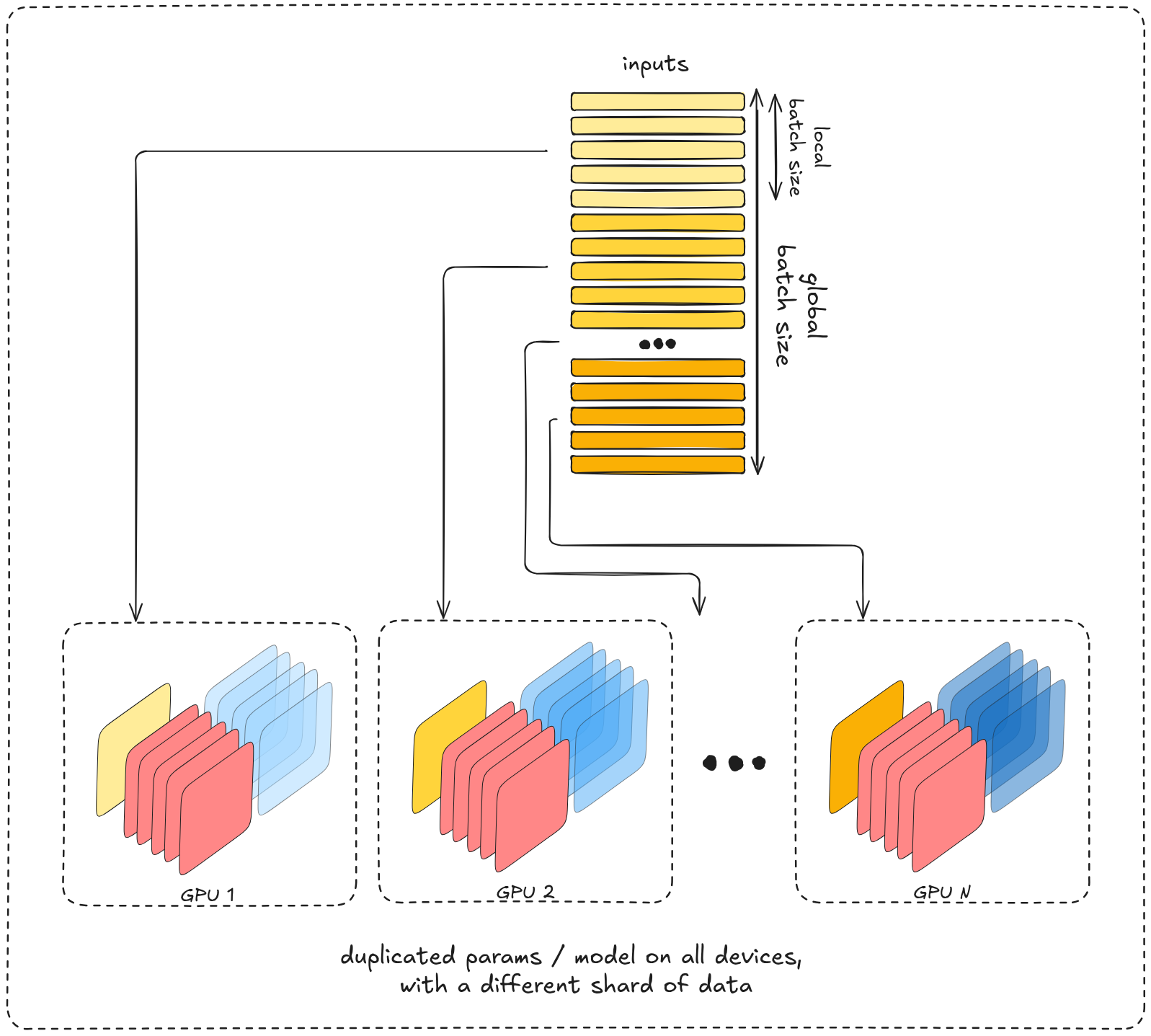
Fully Sharded Data Parallel
the main gain from the Data Parallel approach is that we’re processing a “larger” batch at the same time utilizing multiple devices, the main drawbacks are devices communications which is quite negligeable at this stage since it’s used ~once per batch
the “we can do better” here is avoiding storage redundancy, more specidifcally, we’re currently storing the same model weights replicated on all devices. as discussed earlier we’ve already mitigated the largest memory space (: activations) but we did nothing about the model params memory space, which is still quite significant (varies case by case)
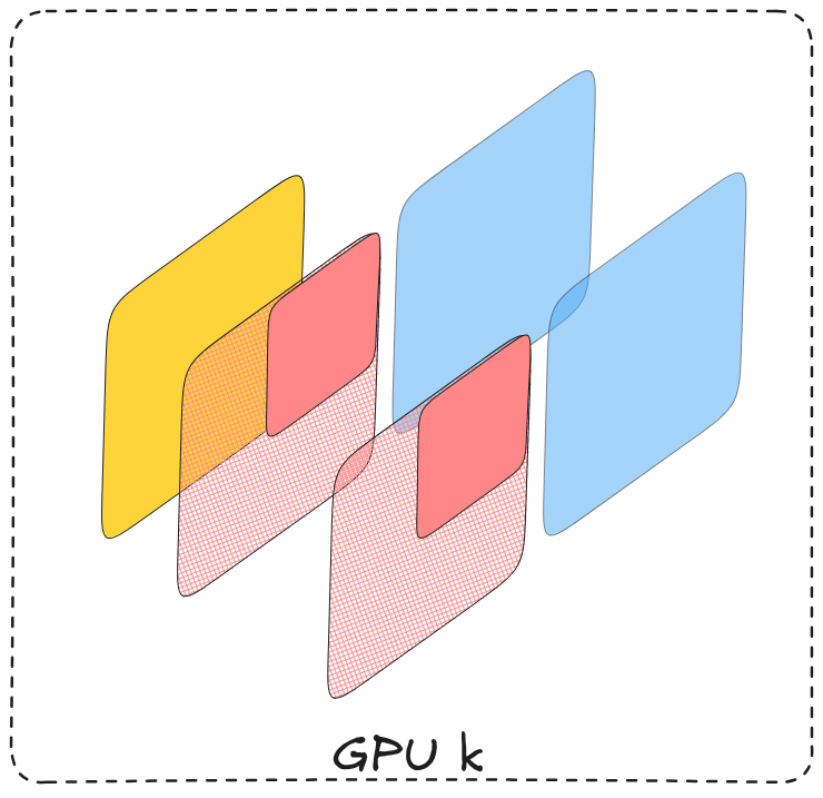
a single device view: a single micro-batch, a chunk of params
the high level idea behind FSDP (fully sharded data parallel) is to not replicate the model parameters across all devices but rather store (mostly) a single copy sharded across them, in other words each device will only store a chunk of model parameters, furthermore sharding won’t be depth wise but rather width wise
:for each block in our model we’ll shard its parameters across all devices instead of replicating’em
initially each device will have as input a single micro-batch, exactly as in Data Parallel, model parameters too will be sharded across devices and not entirely present on each
during the forward pass, for each model layer / block each device will collect the rest of the params tensor in order to compute and store activations of its micro-batch, and then only keep its original chunk of the params tesnor.
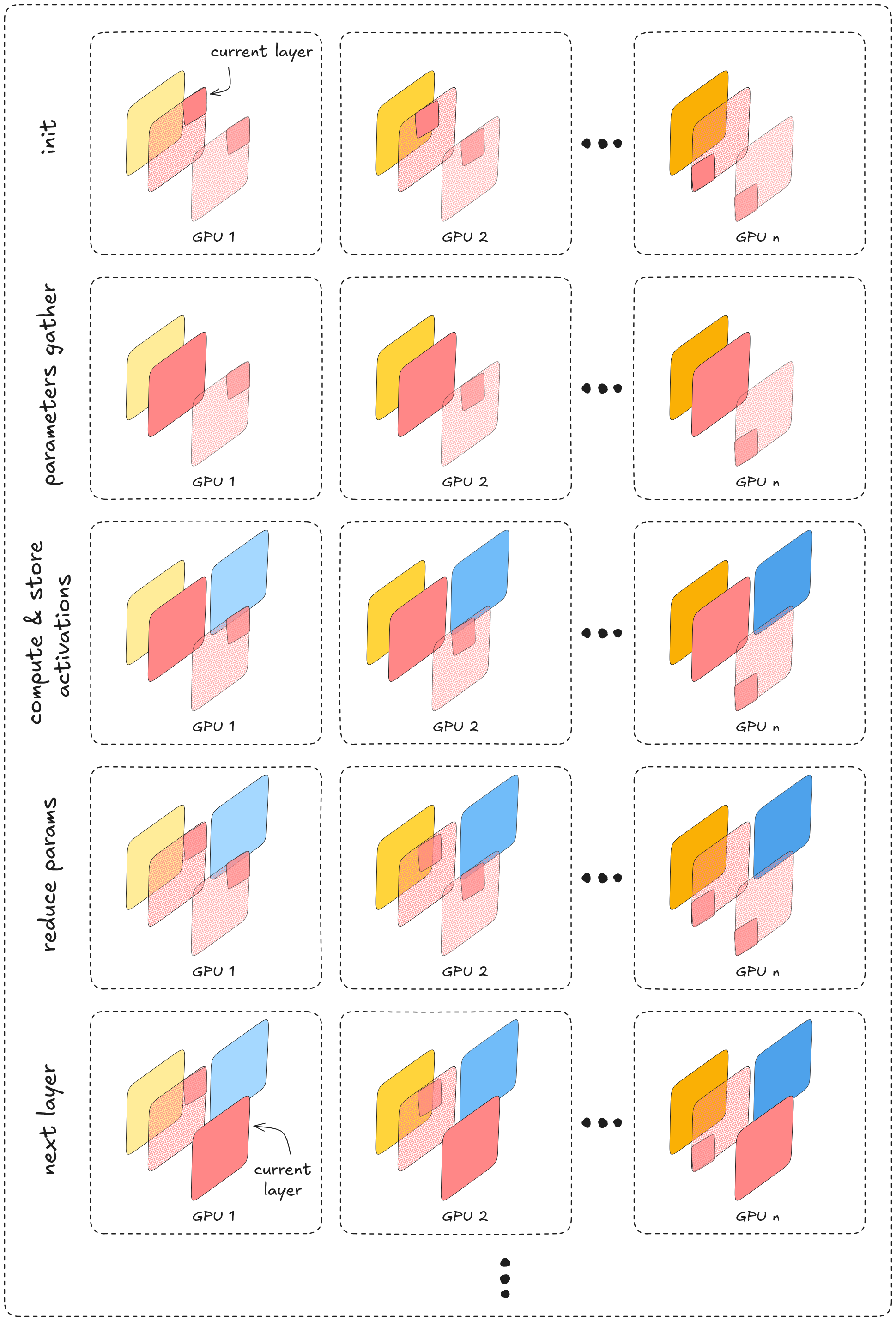
During the backpropagation pass, computation proceeds block by block. for each block, its params are
all-gather
ed in order to apply the global upstream gradient propagated from downstream layers. using that global (all micro-batches) gradient, we compute gradients of the loss w.r.t the block’s activations (for downstream gradient propagation) and with respect to its parameters (for updates / optimization).Once the param gradients for the block are produced, they are
reduce-scatter
ed so that each device retains only the shard of the globally averaged gradient corresponding to its params shard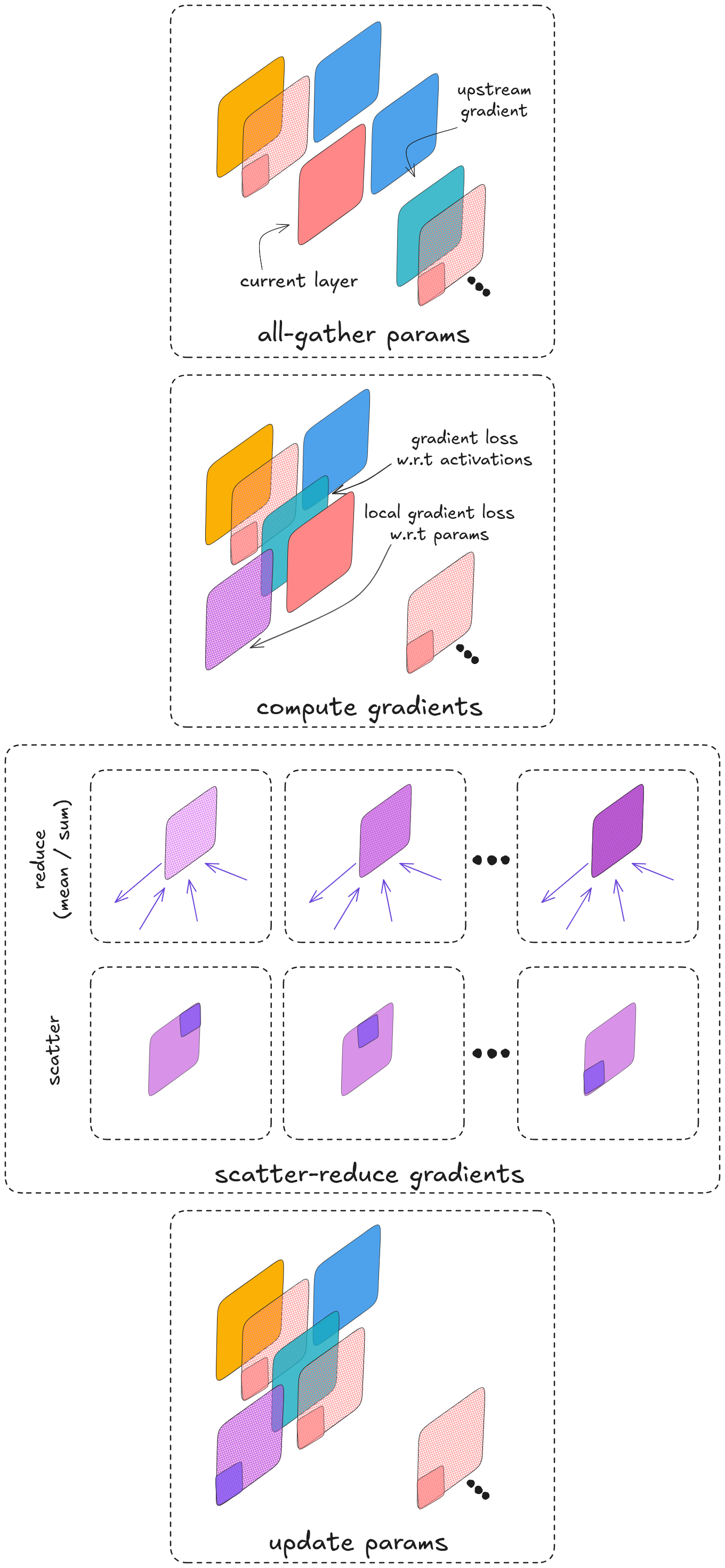
Focusing on evolving from Data Parallel to FSDP, we’re exchanging memory space for communication overhead, to have a better gain-to-loss ratio few tweaks are used in practice.
The main free lunch here is selecting which parameter tensors to shards and which not, for example bias vectors aren’t usually a burden memory-space wise, in contrast to larger tensors. Leading most engineers to only shard tensors larger than a certain threshold to avoid the communication overhead on those relatively small tensors.
Another optimization exploits GPU stream parallelism by asynchronously prefetching the next block’s parameters while computing the current block’s activations, overlapping communication with computation to reduce idle time.
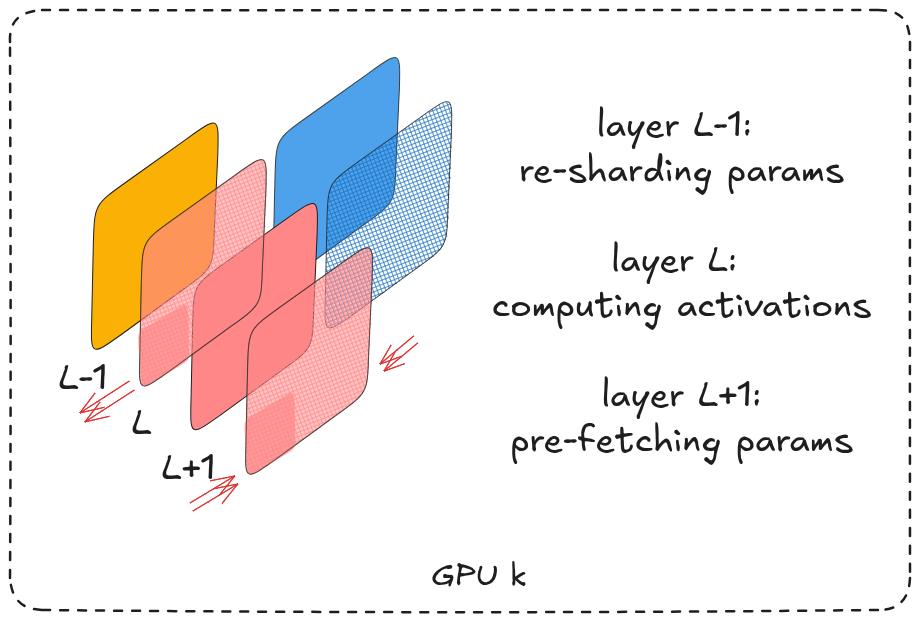
overlapping compute & communication
While FSDP reduces memory pressure by sharding parameters, it still assumes data-parallel execution. A different axis of parallelism is to shard the model itself along its depth.
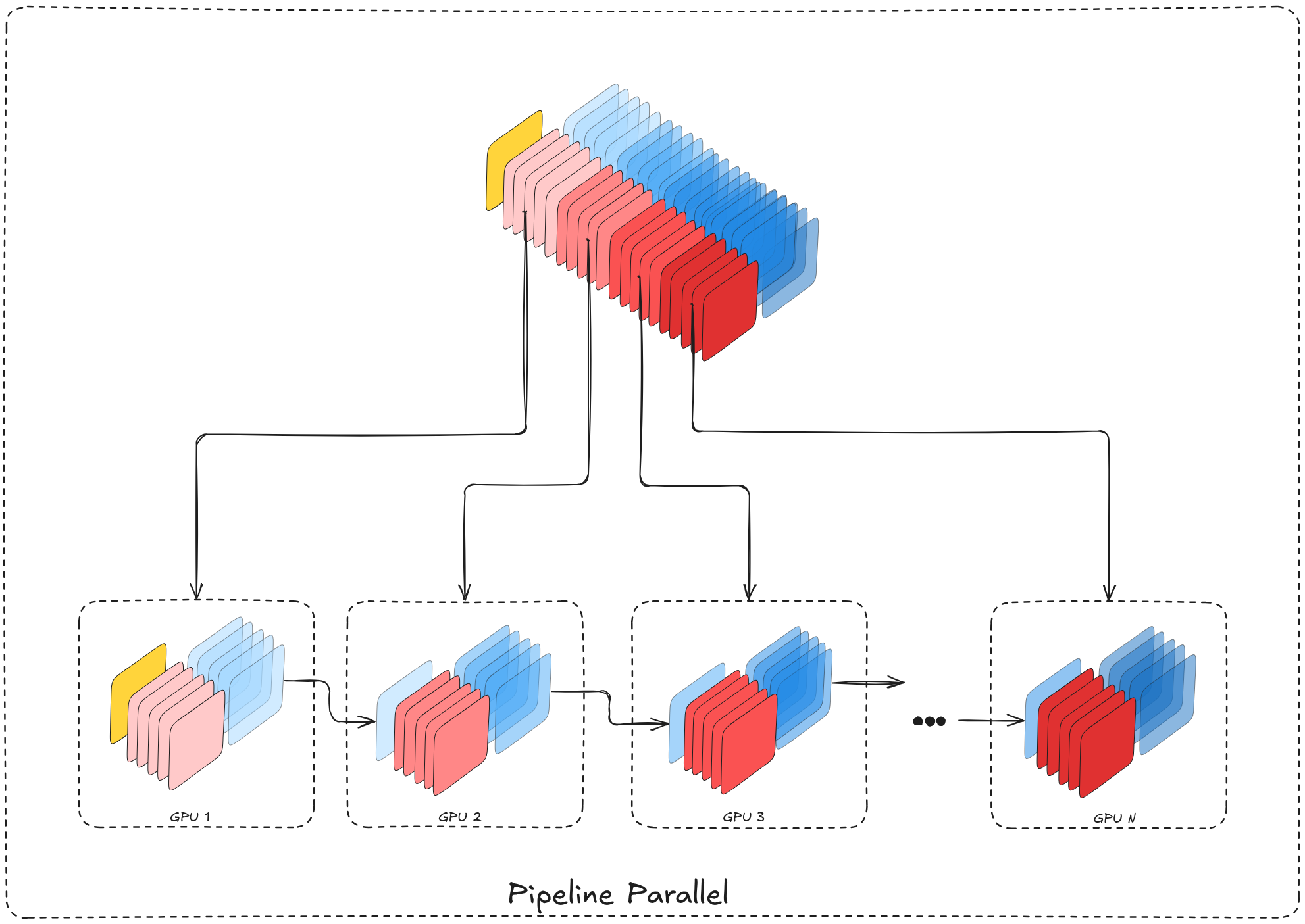
Pipeline Parallel
Another direction to utilize multiple devices for training is spreading them along the direction of data flow, by sharding the model depth-wise on multiple devices. In this setup the model is split into consecutive groups of blocks, where each group lives on a single device. each device, given an input (the previous device’s output), performs its computation and produces an output to be fed into the next device (containing the next group of layers) until the last layer of the model.
Although simple in principle, the sequential nature is the main bottleneck to overcome.
when working with multiple micro-batches the main hold-off of this strategy become clear. In a naive pipline execution fashion where all forward passes are executed first followed by all backward passes, each device will store the activations from each batch until its backward pass is executed which won’t happen until all batches pass the entire model / sequence of devices
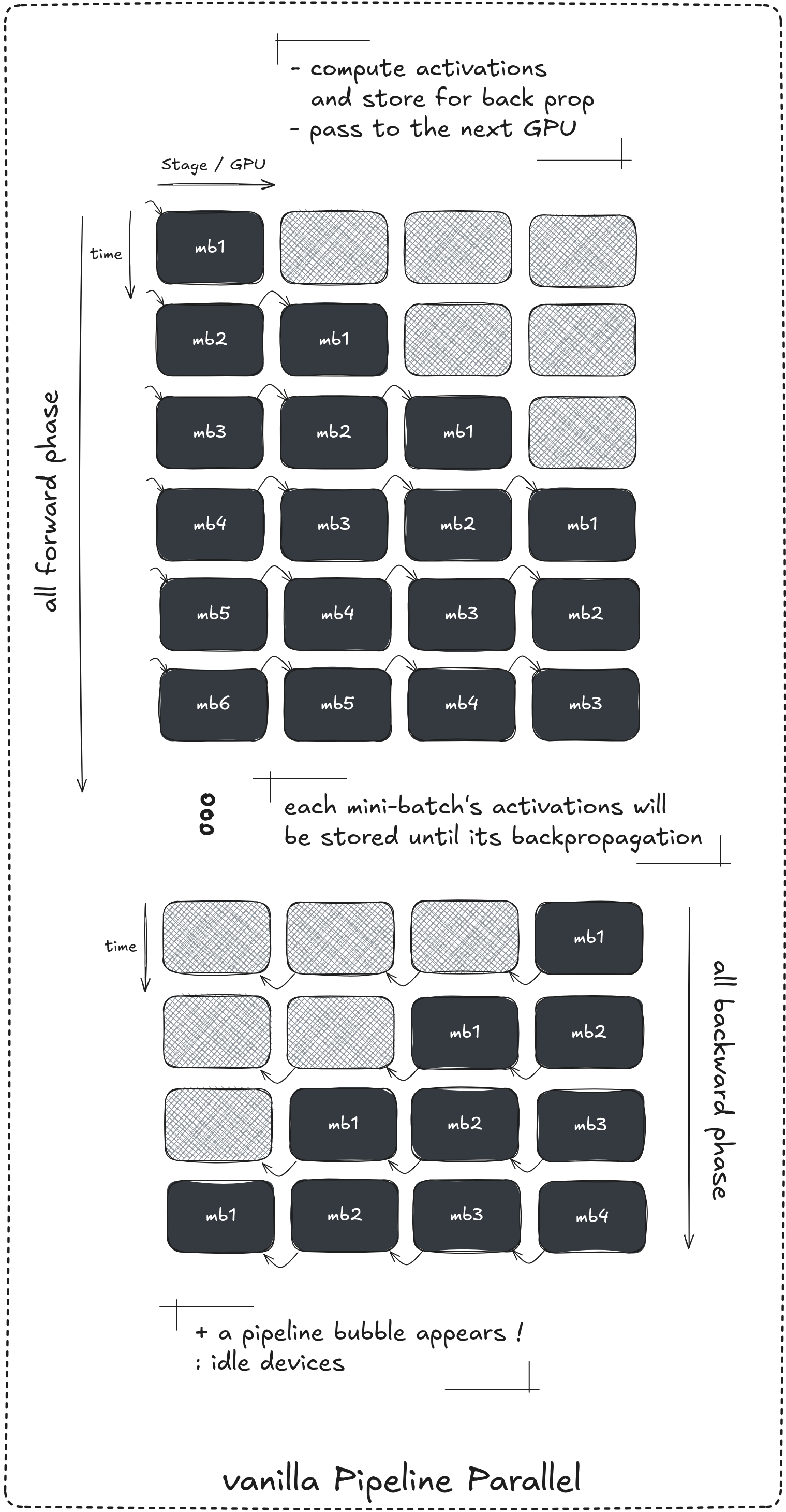
mb: micro-batch*
Along with the memory issue, storing all micro-batche activations until their corresponding backward pass occur, it’s easy to see that depending on the pipeline depth and number of micro-batches, devices become idle during the fill phase of the forward pass, during the transition to the backward pass and during the drain phase. These idle regions are referred to as “pipeline bubble”.
Few variations of the plain vanilla pipeline parallel try to address these issues, we discuss few of them next.
1F1B: one forward one backward
The one forward one backward scheduling strategy aim to reduce activations storage on devices by interleaving forward and backward passes instead of a completely seperating them.
Once the first micro-batch reaches the last device in the pipeline (the filling phase) we enter the new 1F1B phase which simply atlernate between computing a forward pass on all pipeline stages / devices in a timeslote and computing a backward pass on all devices the next one untill the drain phase (when all forward passes are done).
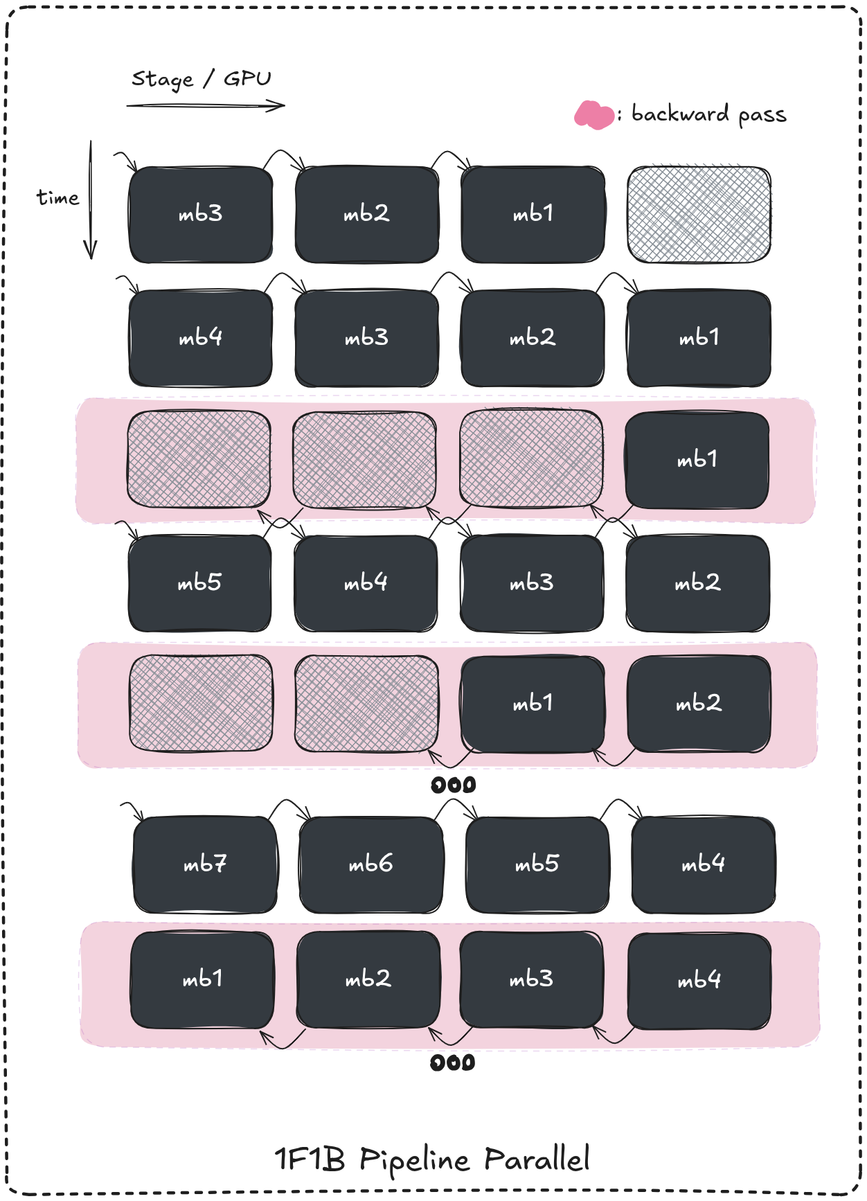
Following that logic each a micro-batches activations won’t be stored for as long as when using the vanilla strategy.
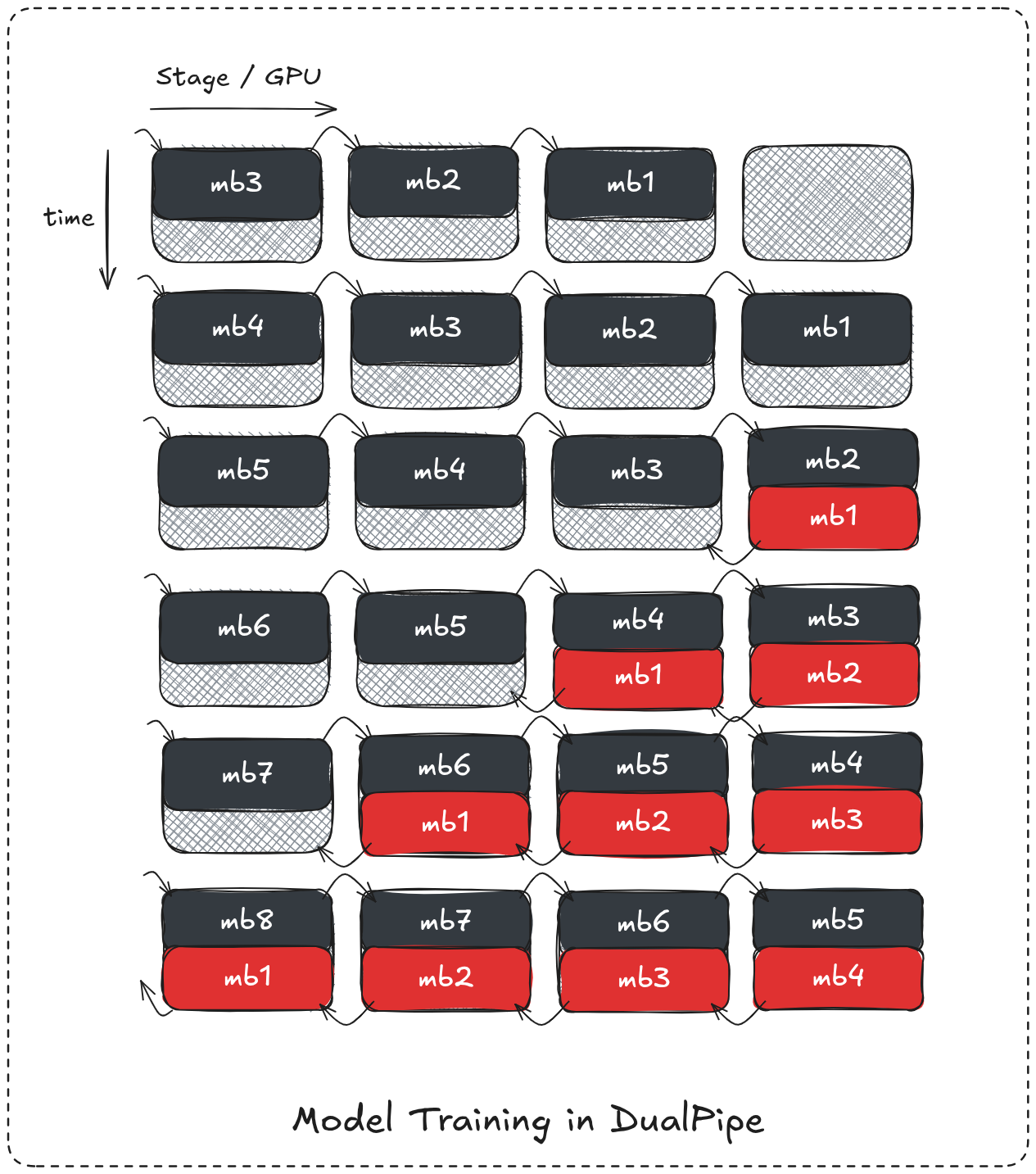
DualPipe
Another interesting approach utilize the device’s streams parallelism to achieve an even better forward-backward overlap. Instead of alternating both passes it assiges separate streams for forward pass computations, and others for backward pass computations and executes them simulatenously.
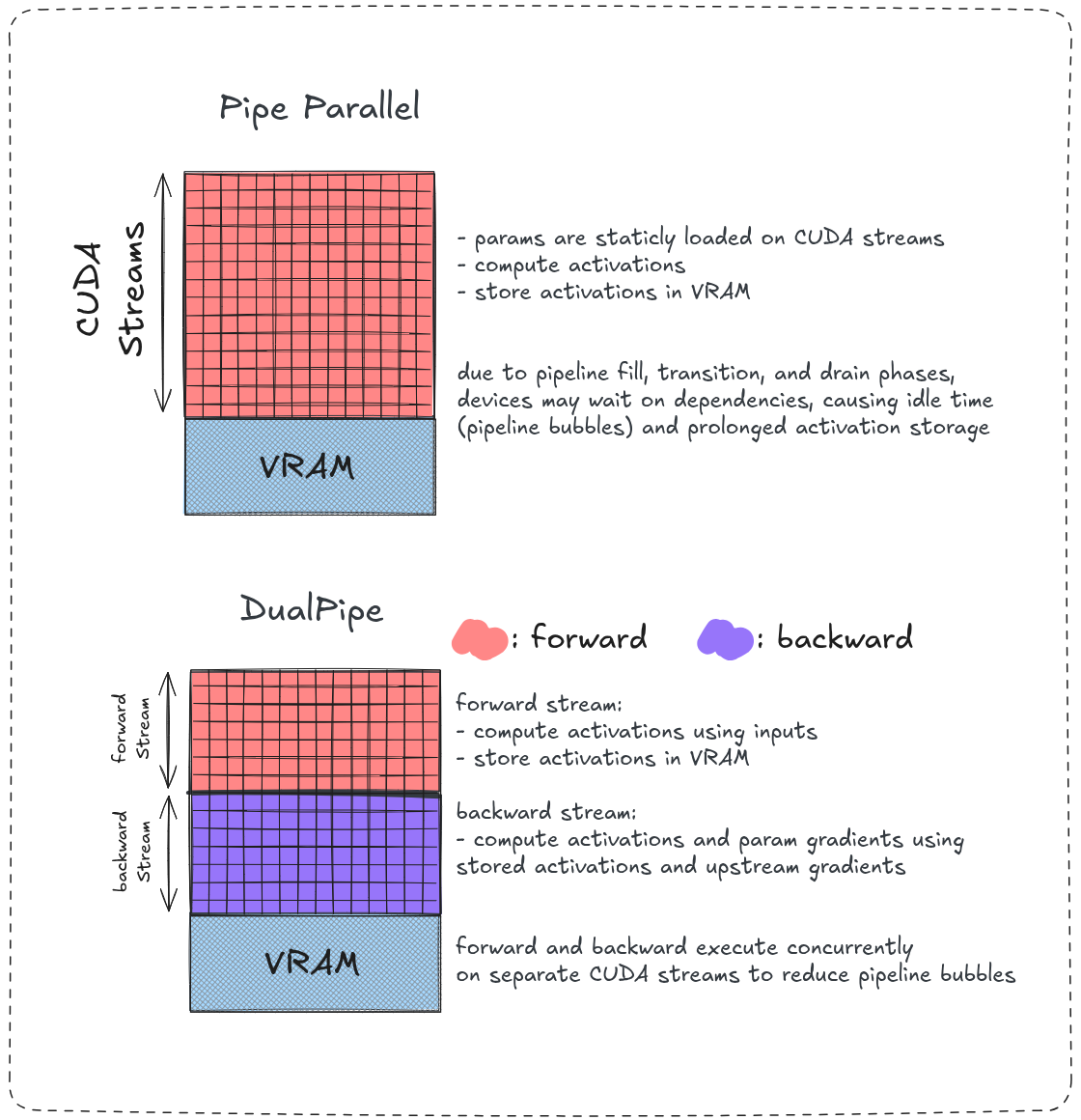
On each device during the forward propagation a micro-batche’s activations will be computed in forward streams and stored in VRAM and at the same time some other micro-batche’s gradients are being computed on the backward stream by the already stored activations achieving a much better computation overlap and an even smaller pipeline bubble.
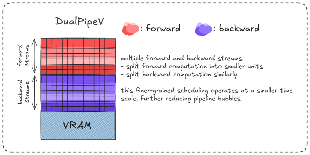
DualPipeV
A slight modification for even better throughput, which further increases overlap by introducing finer-grained stream separation. Instead of using a single forward stream and a single backward stream, computation is divided across multiple “virtual” streams, allowing more granular overlap between forward computation, backward computation and communication.
Notes & Abstractions
A few abstractions are made throughout this blog, that is important to explicitly mention. Other than the already mentioned optimizer state, the main one concerns communication operations, which are treated abstractly in the text. In practice these operations are executed on separate, dedicated CUDA streams and handled by a backend communication library (most commonly NCCL), a detail that is largely consistent across all the distributed training setups discussed here. This abstraction allows the discussion to primarily focus on execution order, dependencies and overlap opportunities rather.