
Introduction
This blog aims to shed light on a relatively overlooked interpretation of neural networks. For simplicity, we’ll focus on classification, but any task falls under the same framing.
Most materials interpret perceptrons as simple decision boundaries in input space and MLPs as forming ever more complex, expressive boundaries by aggregating these simple ones all, always, projected back onto the input data canvas.
Another view, under-explored but equally powerful, keeps the final perceptron as a simple boundary, but not in raw space. Instead, it operates in a learned latent space: the activations of the last hidden layer. Stating that the network doesn't sculpt complex boundaries in pixel space; it sculpt the dataset, point by point, in a new space where a linear hyperplane suffices for our classification task.
One view draws squiggly lines on the original map. The other moves the data using a mapping function (nn) where a straight line set the boundary.
The Classical View: Decision Boundaries Projected onto input Space
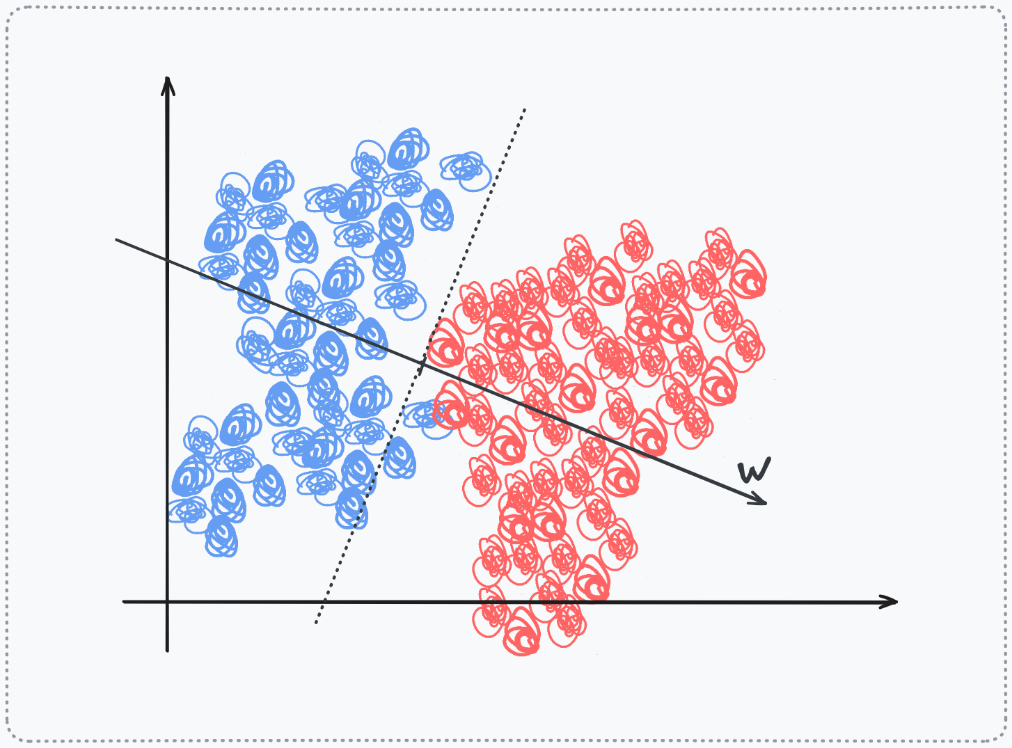
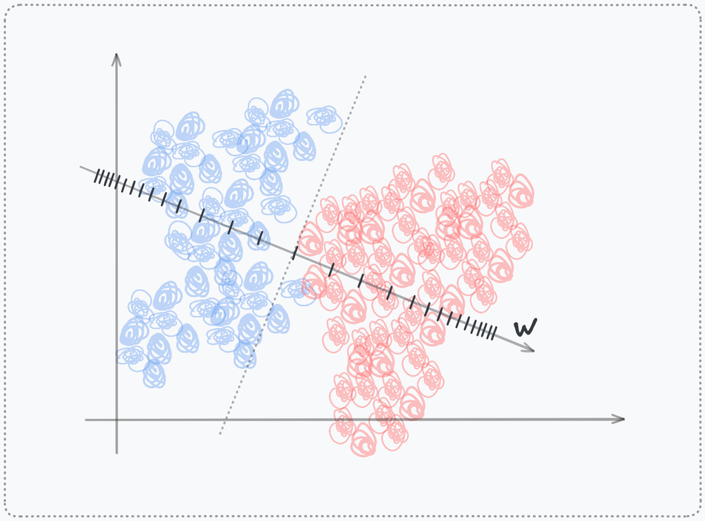
Most materials frame a single perceptron as a decision boundary in the original input space. Given an input vector , a neuron computes the weighted sum . The set of points where <
span aria-hidden="true" class="katex-html">z=0 forms a hyperplane perpendicular to the weight vector , partitioning the raw data space into two half-spaces. That hyperplane is the decision boundary formed by that perceptron
When stacking multiple perceptrons into a layer, each creates its own hyperplane, each oriented differently based on its learned weights. The subsequent layer does not operate on these boundaries directly, instead it receives the signed distances from these hyperplanes as its input. Through its own weighted sum, it creates a new hyperplane, but this hyperplane exists in the space defined by the previous layer's distances, which are then mathematically projected back onto the original raw space. The result is a composition: a boundary that is a non-linear aggregation of simpler boundaries, each defined in terms of distances from earlier boundaries, all ultimately expressible as a complex, potentially fractal surface overlaid on the original input pixel/raw space.
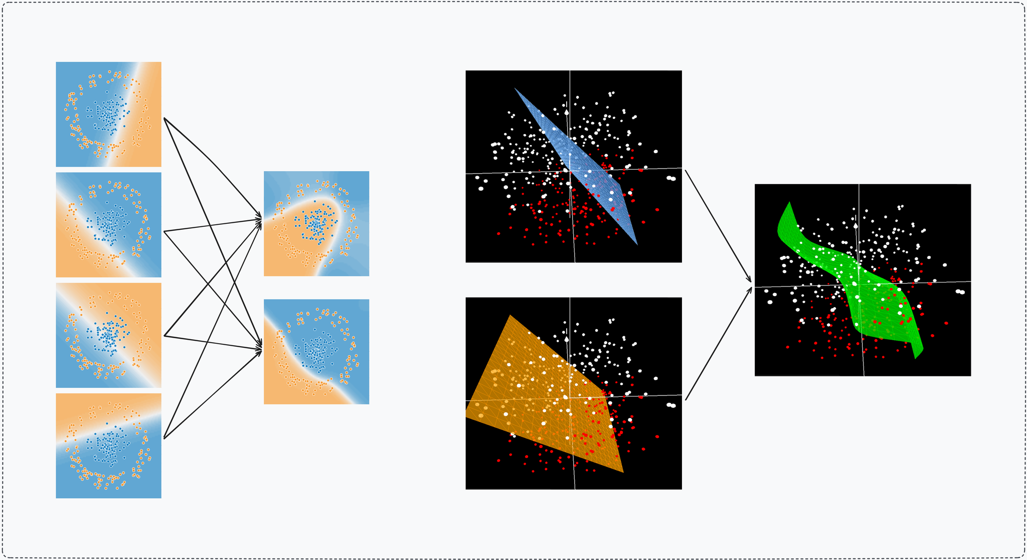
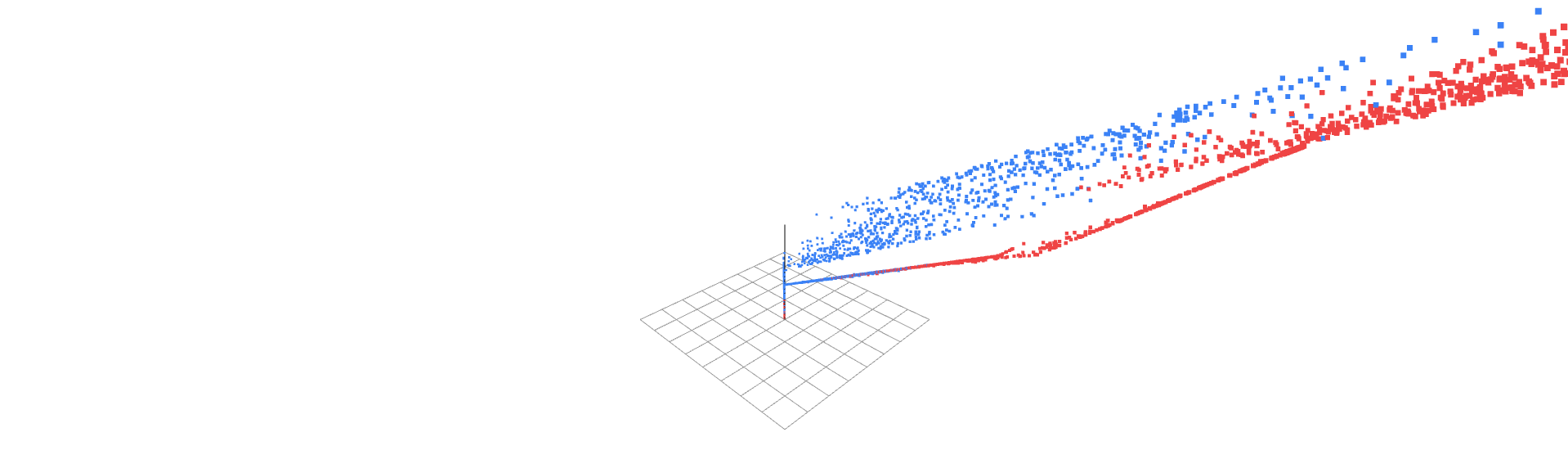
2D vs 3D input space and learned decision boundaries across layers
Activation functions (sigmoid, GeLU, …) enables this complexity, Without it, stacking layers would still produce linear boundaries. Each layer can warp and combine the boundaries of the previous layer, creating curves, loops, and arbitrarily expressive shapes drawn directly on the input canvas. The mental model remains anchored to the input space: we visualize a static data manifold with an increasingly intricate boundary cutting through it.
The Coordinate Transform View: Learning Representations, not Boundaries
Instead of constructing ever-more-complex boundaries on a fixed space, consider an alternative: the network learns a sequence of new representations where simple boundaries suffice
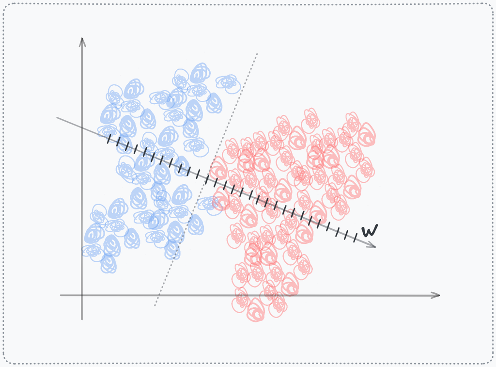
The Perceptron as a New Axis
Take the same computation . Rather than interpreting this as defining a hyperplane in the input space, view z as a coordinate value along a newly forged axis. The hyperplane is merely the origin of this axis. The neuron's output for a data point tells you its position along this axis (signed distances): how far it lies from the origin, in the direction of . The weight vector is the basis vector of this new dimension.
Non-Linearity Warping Axes
The activation function warps this axis non-uniformly. A , for instance, compresses the entire negative half of the axis into a single point (zero), while preserving a linear scale on the positive side. This is not just "introducing squiggles" into a boundary, it fundamentally changes the metric of the new space. Distances along this axis become context-dependent: moving from z = -2 to z = -1 means nothing (both map to zero), while moving from z = 1 to z = 2 represents a meaningful shift.
A activation warps the axis differently but with the same principle. It compresses the entire infinite real line into the finite interval (0, 1), with non-uniform scaling that is strongest at the extremes. At large positive values of z (z > 5), the axis is a flat plateau near 1, incremental changes from z = 5 to z = 6 produce almost no movement along the axis (0.993 → 0.997). The same flattening occurs for large negative values (→ near 0). Only in the narrow region around z = 0 does the axis retain meaningful movement: moving from z = 0 to z = 1 shifts the coordinate from 0.5 to 0.73, a substantial repositioning relative to the axis's entire range. This creates a "focusing effect" where points with moderate weighted sums are thrust far apart along the axis, while points in the saturated regions are locked in place, their distances collapsed to near-zero. In score terms, while enforces a hard threshold between "positive" and "negative", sigmoid creates a gradient from "definitely postive" to "definitely negative," with a wide margin of uncertainty where small differences in input produce large differences in score. The manifold's movement through this dimension is thus highly localized: only points near the axis's sensitive center drift and separate; the rest are mostly cemented into the compressed regions.
linear scale
non-linear scale
Transforming the Manifold
When a layer computes for all inputs, it is not creating boundaries. It is assigning new coordinates to every data point. The entire dataset, previously a crumpled manifold in input space is lifted and deposited into a new space where the axes are these learned, warped dimensions. A point's coordinates in this new space are entirely determined by its location in the previous space; the transformation is continuous and maps the entire manifold at once. The network is sculpting the dataset's manifold shape, not drawing on it. Each layer bends and reconfigures the manifold, incrementally (hopefully) teasing apart the class entanglements.
The Score Function Intuition: What These Axes Represent
These new axes are not abstract mathematical artifacts. They function as score functions for emergent concepts / features.
Consider a neuron computing a weighted sum of features: hours studied, sleep quality, past grades. Its output is a score z = 0.7·hours + 0.2·sleep + 0.1·grades - 5. The activation says: "If the score is negative, the student is not ready (output zero). If positive, their readiness is proportional to the score." This neuron's axis directly measures "exam readiness."
The same applies at every layer. Early layers might compute low-level scores: "vertical-edge-score," "texture-score." Deeper layers combine these into semantic scores: "eye-score," "ear-score." The axes are hierarchical scoring systems, where each score is a non-linear weighted average of previous scores. The manifold moves through spaces defined by increasingly abstract evaluations of the input.
Sequential Sculpting: How Depth Warps the Manifold Differentially
Depth enables compositional refinement. Each layer's transformation depends on the position of points in the previous space, but the effect is not uniform across the manifold.
Non-Uniform Warping and Semantic Saturation
The non-linearity means that progressing from a score of 1 to 2 is not equivalent to progressing from 20 to 21. A score of 1 to 2 might cross a critical threshold (e.g., from "not ready" to "barely ready"), while 20 to 21 might be negligible (from "very ready" to "still very ready"). In spatial terms, this translates to differential motion: points in certain regions of the manifold are slid only slightly along the direction of a new axis, while points in other regions are thrust dramatically forward.
A , for example, collapses all points with negative scores into a flat hyperplane at zero. These points cease to move relative to each other along that axis in subsequent layers. Meanwhile, points with positive scores continue to drift and separate. This creates a folding and stretching effect: some manifold regions are compressed, others are expanded, pulling similar-class points into tight clusters while pushing different-class regions apart.
Layer-by-Layer Manifold Evolution
Layer 1: Maps raw pixels to axes like "vertical-edge-score" and "blue-blob-score." The manifold gently folds; vertical edges cluster on one side of the edge-score axis.
Layer 2: Builds "eye-score" from combinations of Layer 1 scores. Points far apart in pixel space but both containing eyes converge to similar eye-score coordinates. The manifold stretches, pulling eye-regions together while compressing non-eye regions.
Layer L: The manifold is now nearly linearly separable. Cat-images form a dense blob at high values on the "cat-ness" axis; dog-images form a distinct blob elsewhere. The final layer simply places a hyperplane perpendicular to this axis at the threshold where “cat-ness” equals “dog-ness”.
Conclusion: Geometric Reframing gained by this Percpective
This different perspective offers a better view of a network mapping from input to output space convaying depth as a chain of simple transformations and a relative low dimensionality: each dimension is a perceptron in the layer corresponding to a non-linear axis and width as a single transformation with many many non-linear axies corresponding to more warped regions (e.g sensitive range in sigmoid)
It turns regularization into geometry: Overfitting isn't memorization, it's the manifold folding so tightly that tiny input changes launch a point across class boundaries. L2 regularization literally penalizes sharp folds. Dropout forces the manifold to stretch smoothly in directions that don't depend on any single axis. Early stopping halts before the sculpture turns fractal. we're not just "simplifying weights", we're forbidding the transformation from becoming brittle.
It connects every architecture: CNNs build the same local, reusable axes at every image patch. Transformers build the manifold on which tokens will move each others in the communication phase and utilize MLPs for space-to-space transformations following the same low-to-high semantic features intuition described earlier. Both are sculpting manifolds; CNNs use a fixed chisel and eventually aggregate (super) pixel representations, while transformers use one that allows token points in space to communication and move each others. Same principle, different constraint and mechanisms.